Line arrays – X-Treme Audio MISI User Manual
Page 5
5.1 Directivity analysis
The
directivity function enables us to evaluate the pressure distri-
bution in relation to a definite emission direction. By using again the
formulas of fig. 2, the directivity function
R(
α) can be defined as:
where
p
max
is the pressure in the maximum emission direction, in
which from a mathematical viewpoint the exponential function be-
low the integral sign assumes the maximum value (= 1). Following
what has been stated above, one can obtain:
In order to have a qualitative representation of the linear source
directivity, take into account the simplest situation (the so-called
uniform linear source) with a constant amplitude (A(l)=A) and null
phase deviation (
ϕ=0). One will have:
whose solution is:
rendering the wavelength
λ explicit from the expression of the wave
number k.
fig. 3
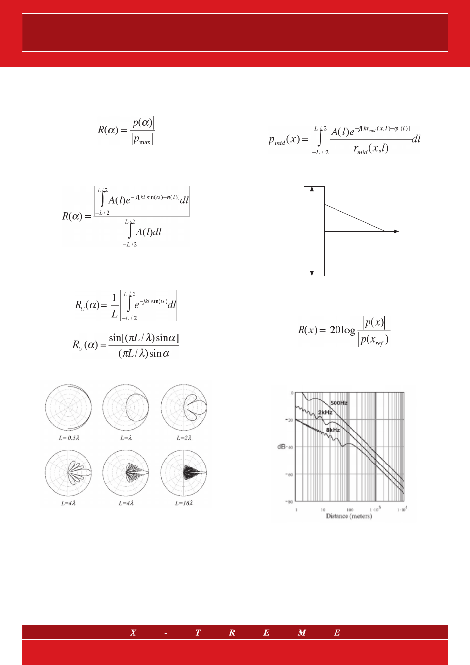
Figure 3 shows the
polar diagrams of function R
U
(
α).
Let’s consider the
L/
λ
ratio (0.5, 1, 2, 8, 16), i.e. the ratio between
the line length and the wavelength. It can be easily noticed that a
very high directivity is obtained in wavelengths that are much short-
er (1/8, 1/16) than the line length (in the specific case of a few metre
long line arrays, this leads to mid-high frequencies). In other words,
in the case of a linear source, the narrower the main emission lobe
is, the better the sound energy transmission can be forced into a
narrow and orientable corner of the sound front.
5.2 In-axis response analysis
Similarly to the directivity analysis, and referring to fig. 2, we force the
(observation or “listening”) point P to lie on the axis x. Now let’s go
back to the general case, thereby excluding the far-field hypothesis.
The pressure form will therefore be of the following kind:
where r
mid
(x,l) is the distance traced in fig. 4
dl
p
mid
(x)
x
Line source
L
P
r
mid
(x,l)
fig. 4
The corresponding directivity function on the x axis is often expres-
sed in a logarithmical form:
Where x
ref
is a reference distance, generally 1 m.
Note that R(x
ref
)=0. The double logarithmic graph of r(x), in the specific
case of a 4 m long uniform linear source (as already seen in A(l)=A and
ϕ=0), will have a qualitative trend of the type shown in fig. 5
fig. 5
Each curve refers to a certain sinusoid frequency. A double slope is
observed for each curve: as the distance from the source grows, at the
beginning there is a decrease of 3 dB for each doubling of the distance,
then there is a decrease of 6 dB for each doubling of the distance.
The (theoretical) point in which the curve changes its slope is called
transition distance and it is a function of both the fre quency and the
dimension of the line source (
L). The branch with a -3 dB slope is the
near field, that with a -6dB slope is the far field.
5/21