X-Treme Audio MISI - Manual (Page 3)

LINE ARRAYS
2. Sound power and pressure levels
At present, one of the most common and interesting problems to
face is the following: let the
sound power (or the sound power level)
of a certain source be given, a magnitude that characterizes it intrin-
sically, determine the
sound pressure (or the sound pressure level)
at any point of the space where the source works. In a free field
or in a free field on a reflecting surface, this problem can be easily
solved by calculating all the necessary elements with the following
simple formula:
Lp = Lw + ID
θ,ϕ
- 20 log(r) - 11 [dB].
Therefore this relationship, which is valid in far-field conditions (in fact,
in this case all the real acoustic sources smaller than the wavelength
of the sounds they produce can be approximated as pulsating point
spheres known as “monopoles”), enables the calculation of the
sound
pressure level Lp produced by a source having a sound power level
Lw (=10 log W/Wo with Wo= 1 pW; e.g. if the acoustic power of a speak-
er system is 100 W its sound power level will be 140 dB), at a certain
distance r in a direction such that the di rectivity index of the source is
ID
θ,ϕ
(=10 log Q
θ,ϕ
with Q
θ,ϕ
being the direc tivity factor of the source in the
direction identified by angles θ and ϕ).
For example, a source with a sound power level of 120 dB (there-
fore with power W equal to 1 Watt) and a directivity index of 3
dB in the direction where the listener is positioned, produces a
sound pressure level of 84 dB in a 25 m far free-field, because:
Lp = 120 + 3 - 28 - 11 = 84 dB.
Furthermore, if we know the sound pressure level Lp
1
at a certain
distance r1 from the source (for example, by measuring it through
a sound-level meter) and in a certain direction, the sound pressure
level Lp
2
can be determined at another distance r
2
in the same di-
rection, without necessarily knowing the sound pressure level.
In fact, by using the equation above, we obtain:
Lp
2
= Lp
1
- 20 log(r
2
/ r
1
) [dB].
If, for example, a source produces a sound pressure level Lp
1
=
92 dB at a distance r
1
= 8 m, the sound pressure level at r
2
=16 m,
in the same direction, will be 86 dB (as mentioned at the begin-
ning, the sound pressure level decreases by 6 dB when distance
doubles).
Note: in a free-field on a reflecting surface, in the semi-space where
the source is forced to radiate, as previously mentioned, the sound
intensity is twice the intensity existing in a free field. Therefore, 3 dB
should be added to the sound pressure level calculated with the
formula above.
3. Physical-mathematical model: brief description
Most acoustic models are simplified solutions of a general equation
(
wave equation) which are subject to certain “constraints”, such as
the environment’s volume or its known value at certain points in the
listening space. Therefore, in an acoustic study the used formulas
are a small set of specific solutions which is almost suitable for de-
scribing with sufficient approximation the acoustic field in a listening
environment. In general, these solutions are expressed in terms of
pressure in relation to space and time variables.
In
indoor acoustics, the space characteristics are modelled as
boundary conditions and they exert a remarkable influence on the
acoustic field. It is the physical dimension of the space that makes
the presence of waves with a certain length possible (or impos-
sible). In mathematical terms this falls within the category of the
eigenvalue problems. The solutions will be strictly dependent on
frequency and will have periodical behaviours (in acoustical terms
this is the so-called modal theory).
On the contrary, in outdoor acoustics, the boundary conditions
imposed on the wave equation will commonly be radiation condi-
tions, which are necessary to make the mathematical model coher-
ent with the physical reality. The dependency on frequency is no
longer regular as it occurs in closed spaces and the modal theory
cannot be applied. Of course, the differences between open and
closed spaces affect sound reproduction and the ability of a speak-
er system to adjust to different reproduction contexts, especially if
we consider the wide range of problems arising in open spaces.
Line arrays can solve the various problems associated with
sound reproduction. In this short introduction we will analytically
describe a line array mathematical model and we will com ment
on a few important results deriving from this model. Finally we will
demonstrate that a simple theoretical model can suitably meet
the coherence requirements with real measurement. This short
introduction, having an analytical and general character, will not
deal with the problems concerning the technological features of
the models (waveguides, etc…) or with the electro-acoustics so-
lutions that are nevertheless essential for designing and produc-
ing line arrays.
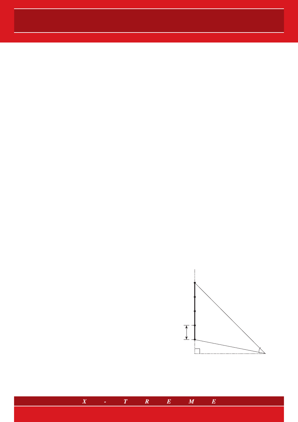
4. Linear sources: introduction
Generally speaking, real sound sources are very complex and it
is quite difficult to describe them in detail. Luckily, in most practi-
cal cases, we can resort to substantial simplifications. The most
drastic one, as previously mentioned, consists of considering a
real source as an infinitely small point source whose dimensions
are actually much smaller than the wavelength
λ of the reproduced
sound and/or if the listener is at a great distance from the source
position. However, other more complex ideal sources can better
represent the properties of the real sources: it is the case of the
linear sources, namely point sources that are conveniently ar-
ranged along a straight line, which are used in the literature to
exemplify a stacked or flying
vertical line array system. A row of
cars along a straight road is another more common example of a
real source which can be approximately represented as an infinite
length linear source.
n
...
3
2
1
b=step
90°
W
0
W
0
W
0
β
η
r
0
P
Line source
fig. 1
3/21