X-Treme Audio XTI - Manual (Page 4)

User’s guide
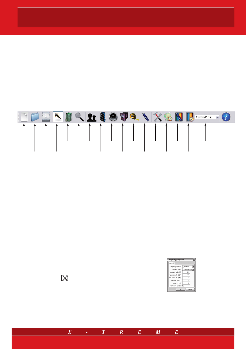
new
project
select zoom new
array
new
sub
trace
section
SPL
calculator
autorange
map
band
select
open
project
save
project
trash new
audience
new
speaker
“meter” setup global
autorange
Entering a higher than native resolution (third octaves) the user can
obtain more accurate and homogeneous maps, because differ-
ent interference patterns arising from a greater number of varying
frequencies (each of which is possibly present in the actual signal
reproduced) overlap.
Listener height: the generic height of the listener in meters. It is used
in zones in which no audience areas are set (see next paragraph).
Max and Min map values: expresses the upper and lower limits
in dB of the range used in the section view (and map view if Autor-
ange is not set for the map view, see Autorange explanation below)
corresponding respectively to the warmest and coldest color in the
color-bar for broadband views (“Lin” or “A-weighted”). The scale
for single octave visualization is automatically lowered by 10 dB be-
cause, in the presence of broadband signals, the energy contained
in an octave is on average one-tenth (-10 dB) of all of the acous-
tic energy present. When any new data is entered, the Autorange
function on the main screen is disabled and the next map will be
calculated with the new range set manually.
Temperature: enter the estimated air temperature during the per-
formance (in Celsius) here. In the calculation, the temperature influ-
ences the sound speed and the resulting interference pattern.
Humidity: enter the estimated air humidity during the performance
here. It affects the absorption of sound by the air (important at high
frequencies).
Consider obstacles: if enabled, this option considers audience
areas, represented by four-sided plans, as obstacles. This means
that on each point of the map, the contribution provided by the
speakers that are visually hidden in these plans is neglected. A
geometrical optics estimate is used, which means that diffraction is
ignored. Despite this, the option can be useful if its limits are taken
into consideration. When the option is disabled, audience plans
are acoustically transparent. This function works also if the areas
concerned are switched to “not active” (see below).
Fig. 3 Setup menu
The sound level in each of the plots previously described may be
broadband or limited to a particular octave.
The spectral resolution of the image is thus set to octaves; this
is just a “smoothing” of the internal data, which is calculated at a
higher frequency resolution set by the user.
The plotted SPL is interpreted as the maximum RMS Sound Pres-
sure Level which the loudspeaker system being used can provide.
Subwoofers are also modeled in XTI. It is important to note that the
SPL created by subwoofers is strongly influenced by the environ-
ment, which is currently not considered at all by XTI (for instance,
there is a substantial difference in SPL when subwoofers are placed
on the ground compared to when they are suspended, a difference
that is much less dramatic for normal speakers). Moreover, it can be
misleading to represent the perceived SPL at very low frequencies,
especially when limiting the spectral resolution output to octaves.
And even when we estimate it, it is a matter of experience to de-
cide if it is sufficient, since it is not necessarily aligned with the
response of higher frequencies, but depends on the musical pro-
gram (Fletcher - Munson curves describe this phenomenon very
well!). For this reason, XTI is currently not designed to accurately
suggest the correct number of subwoofers for an installation, nor
is it intended to provide a truly meaningful absolute SPL at those
frequencies. An estimate of the number of subwoofers to be imple-
mented, once it has been given a certain configuration of satellites,
is suggested by X-Treme based on other guidelines, which do not
take the use of XTI into account (see the HPS or Line Array man-
ual). However, this tool is very useful for detecting SPL variations
across the listener area, due to interference, which is very strong
and difficult to handle at low frequencies.
Now, let’s discuss XTI’s unique functions: if you own XTI and have a
PC, turn in on and try it out while reading this document.
3. The toolbar
Figure 2 is an image of the toolbar with a description of the function
of each tool.
4. Setup
Clicking on the icon
opens the Setup menu, which shows the following elements that
can be edited.
Frequency analysis: this lets the user set the frequency resolu-
tion for the calculation. For third octaves, the program performs its
calculations directly on the input data of the file (since it is stored in
third octaves). For higher resolutions, the input values of the files are
evenly divided in the sub-bands that were created.
Fig. 2 XTI toolbar
4/9